Networked New Orleans
This is an excerpt from a longer piece.
Introduction - why networks?
“The dealers’ names were everywhere in antebellum New Orleans: Theophilus Freeman, Jonathan M. Wilson, Bernard Kendig; John White, Calvin M. Rutherford, and Joseph A. Beard. The walls of the city were patched over with their posted bills, the newspapers punctuated by their graphic advertisements, and the coffee shops and saloons overhung with loose and speculative talk about their business. The interstate traders were the best known: Franklin and Armfield of Virginia, the Woolfolk and Slatter families of Maryland, the Hagans of South Carolina.”
As historians, we spend our time reinterpreting sources; we ask new questions of and find new meaning in old material. This essay is an attempt to reinterpret one particular source: a spreadsheet of around 14,000 slave sales which took place in New Orleans from 1856 to 1861. Charles W. Calomiris, a Columbia economist, and Jonathan Pritchett, a Tulane economic historian, compiled the data to demonstrate how slave prices changed in response to the political events immediately before the Civil War; but the data can be used to do much more than that. Calomiris and Pritchett, like many economic historians before them, made a decision to see the market as a list of prices; but while this decision has had useful results, it’s not the only one that could be made. Rather than focusing on prices, I want to see transactions as a link between two individuals; collectively, these links form a network which represents the New Orleans slave market.
Calomiris and Pritchett constructed a massive edifice of regressions and time series to find signal in the noise of their price data. These methods rely on complicated mathematics and have been refined over decades of use; but in this essay, I’m going to use a class of methods called exponential random graph models which have been applied in sociology, but not (as far as I know) in history; these methods can be used to identify topological structures which are peculiar to the slave market. It appears that the slave market has a quasi-bipartite structure, which distinguishes it from the canonical models of network science.
Historians haven’t made much use of networks before; certainly, they haven’t been used to understand antebellum slavery. However, being different is not a virtue in and of itself; the established methods tend to have become established precisely because they’re effective. It’s the reverse of Chesterton’s Fence; if we find a road without a fence across it, our first instinct should not be to say “Ah! I’ve identified a gap - there’s no fence here! I’ll build one right away.” But increasingly the reasons not to see the slave market as a network are falling away: it’s intuitively and visually appealing to imagine the set of traders and the relationships between them in this way, and it’s now computationally feasible to do so. So much of what I’m going to argue in this essay comes from this basic intuition that we should start by getting into the network itself. However, a visual presentation of the full network of 8287 individuals connected by 8501 trading relationships would be a meaningless hairball; and while many of the statistics I’m going to use are calculated on the entire network, exponential random graph models only work with networks of a few hundred nodes. As such, I’m going to focus on the 155 individual actors (some of which are companies), connected by 214 links, who traded for slaves collectively worth at least $20,000.
You can click on individual nodes to highlight their names and connections, and drag them around to see them in more detail. The edges are directed and weighted - an arrow from X to Y means X sold at least one slave to Y, while the shade of the arrow reflects the total value of X and Y’s trades (the greater that value, the darker the arrow). Colour represents the type of state indicated as the “state of origin” on notary records; node size indicates the total value of trades made by that individual.
Presenting what is at some level just a spreadsheet full of names and numbers in this way shows how changing the format of a source can change its meaning; when you start to explore the market as a network, you notice that each node has its own pattern of connections, connecting in turn to nodes with their own patterns. The visualisation itself suggests questions which are not just hard to answer with a spreadsheet, but probably would never be asked in the first place: who interacted with whom, and why? What made a trader choose to buy a slave from one person, and not another? How likely were two people to trade with each other? What roles did individuals play in the market; what roles were there to play? Could everybody trade with everybody else, or did trade have to flow through a few central points? The most important thing is not to constrain ourselves by only asking the sort of questions that can be answered by the data as a spreadsheet; instead, we should be as creative as possible with the presentation of the data, and then follow up the questions that arise.
This analysis focuses on the slave-traders named in the Calomiris data; but there’s not a lot of biographical information about them in the data itself. This biographical information does exist, in personal papers and suchlike, but without access to that, the best I could do was to use Ancestry.com to collate all the available census records about the individuals named in the data. The details about birth, wealth and occupation contained in these records gives a ‘ground truth’ for arguments about the network itself.
We can use the network to make two sorts of comparisons. Ideally, we’d be able to make historical comparisons; I’ve assumed that the period 1856-1861 constitutes a single historical case, but we could make a diachronic comparison to 1830-1831 (for which some good data does exist), or the period before the professionalisation of the slave trade around 1820. We might also compare the market in New Orleans (an importing port) to Baltimore, Norfolk and Alexandria, ports from which slaves were exported, or with Natchez, the entrepôt on the Mississippi to which slave coffles were driven overland.
However, the Calomiris data is of unusual quality: records survive because Louisiana’s 1806 Code Noire stipulated that slave transactions should be notarised like real estate, and have been digitised specifically for Calomiris and Pritchett’s project. As such, although there is data available for other time periods, other markets, and other counties in Louisiana, it’s not been systematically made available.
We can, however, compare the slave market to theoretical network models which have been validated in other fields. The particular strength of the exponential random graph models is that they can be used to generate simulated versions of the New Orleans slave market. These simulations work like counterfactuals; they can show which aspects of the slave market were peculiar, peculiarities which can be explained with historical arguments.
Quantifying the slave trade
Robert W. Fogel and Stanley L. Engerman’s Time on the Cross casts a long shadow over the historiography of the antebellum slave trade: with innovative methods, a dataset of slave trades covering the entire period from 1804 to 1862, and some shocking conclusions, Fogel and Engerman forced two generations of scholars to engage with their ideas. These generations have done so in their own ways; the first responses dealt with Fogel and Engerman on their own terms, refuting their arguments by introducing new quantitative evidence and challenging their methodology. For example, Michael Tadman’s 1989 book Speculators and Slaves focused on the question of family breakup:6 notably, he said that 60-70% of slaves were transported from the Old South to the New South by traders, as opposed to planters migrating their entire estates - not the 16% suggested by Fogel and Engerman, which would have suggested a far lower rate of family breakup.
More recently, however, scholars have focused on the experience of the slaves who endured the journey and the markets: in a movement exemplified by Walter Johnson’s 1999 book Soul by Soul, an exploration of the New Orleans slave markets which focused on the strategies employed by slaves to shape their own sales, writers like John Hope Franklin, Loren Schweninger, and Damien Alan Pargas have sidestepped the quantitative controversies to focus on cultural and social aspects of slave life.7 This has been effective not least because a quantitative approach requires the historian to focus as much on the speculators as on the slaves themselves. Ship’s manifests, probate records, census data, and certificates of good behaviour were created by and for white Americans; these historians have turned to other sources to excavate subaltern voices.
The quantitative historiography of the slave trade has hinged on the availability of data. Time on the Cross was revolutionary partly because it introduced a new dataset, the New Orleans Slave Sample 1804-1862; this has been used extensively by later historians, such as Laurence Kotlikoff in his 1979 article ‘The Structure of Slave Prices in New Orleans, 1804-1862’. While the sample has allowed historians to explore the age profiles and prices of slaves sold in New Orleans, it has its weaknesses: it includes only 2.5-5% of the slaves sold in any given year (giving 5009 observations of 47 variables), and only lists traders by their initials. As such, it only really contains data about price and age, and can’t be used to make inferences about individual slave traders.
A second burst of activity followed Herman Freudenberger and Jonathan Pritchett’s 1991 article ‘The Domestic United States Slave Trade: New Evidence’; the importation of slaves into Louisiana was banned between 1826 and 1828, but the conditions of the repeal of this act meant that, for a brief period between 1829 and 1831, slaves imported into New Orleans had to be accompanied by a ‘certificate of good character’, which supplemented sale records. These certificates gave Freudenberger and Pritchett enough material to construct a dataset of 2,289 slaves imported in 1830; notably, this is a complete record of the surviving data, not a limited sample. This new data supported Tadman’s claim that up to 70% of slaves were imported by slave traders, but disagreed with the explanations that Tadman and Laurence Kotlikoff provided for seasonality in the market. Freudenberger and Pritchett aren’t the only people to have used their dataset; several articles have been written with it over the last decade.
But while Calomiris and Pritchett published their article and dataset in 2016, their narrow, albeit sophisticated, project has not exhausted the possibilities offered by the dataset they constructed; while the 1804-1862 sample and the 1830 certificates were used by various historians for a range of different purposes, no other paper has been published using the Calomiris data; this presents a clear opportunity.
Developments in the study of the slave trade have followed the publication of data; in contrast, the statistical methods employed by economic historians have merely been refined since the 1970s. Tadman’s argument about family breakup was based above all on new data he had collected, while the same is true of Freudenberger and Pritchett’s arguments about transaction costs. The opportunity, therefore, is to marry an under-utilized dataset with a new theoretical approach.
Selecting a sample
Calomiris and Pritchett’s dataset contains “all slave sales recorded in the New Orleans Conveyance Office between the dates October 1, 1856 and August 31, 1861.” It’s clear, however, that this data isn’t actually complete. Richard Tansey, for example, found evidence in personal papers of 758 trades made by Bernard Kendig throughout the 1850s, but only a few hundred of those appear in the Calomiris data, and several individual trades cited by Tansey which fall into the period don’t appear in the data. However, this isn’t an insurmountable problem if the missing data is uniformly distributed; it just means that, if two nodes form an edge with probability p, we will systematically underestimate p. A further crucial point is that these are just the records of Orleans Parish, but trades between neighbouring planters would have been recorded locally. As such, the data records only the trade which passed through New Orleans, not the full picture of these individuals’ actions.
In its original form, the dataset contained 14,850 observations; after dropping empty rows and observations from outside the time period, we are left with 14,462 rows. Calomiris and Pritchett wanted to collect information about the market prices of slaves; as such, they dropped 4163 records for two main reasons: the price information was inaccurate, or the sale did not represent a market transaction. However, because we are interested in the existence of trading relationships, and precise dollar values will be elided anyway, we can include some of the trades that Calomiris and Pritchett omitted. On the other hand, Calomiris and Pritchett included estate sales, which occur after the death of a slaveowner. These were made at market prices, but clearly aren’t an accurate representation of normal market behaviour, and thus I dropped them. After this process, 13,389 observations remain. I also took a lot of care with record linkage in both the Calomiris and census data - making sure that various versions of a name were consolidated into one, without accidentally combining two separate individuals.
Joining the dots
“Where do these networks come from? In some cases, they are the traces of what happens when each participant seeks out the best trading partner they can, guided by how highly they value different trading opportunities. In other cases, they also reflect fundamental underlying constraints in the market that limit the access of certain participants to each other. In all these settings, then, the network structure encodes a lot about the pattern of trade, with the success levels of different participants affected by their positions in the network.”
Networks are extremely complicated objects. There are 2n(n−1) possible directed networks with n nodes; this means that we can connect 10 nodes into a network in over a decillion (1033) different ways, while the 155 individuals in the network I’m going to focus on can be connected in 107185 different ways. This complexity places serious limits on the analysis we can do with networks of a given size.
The formal study of networks traces back above all to the work of Paul Erdős and Alfréd Rényi in the 1950s; under their model, edges form between nodes with probability p, which means that the probability that a given node is connected to k other nodes follows a Poisson distribution:

Their model produces graphs like this:

But while the Erdős-Rényi theory is a decent starting point, real-life networks don’t look like the one above. Instead, modern network science stems from two paradigms identified around the turn of the millenium: friendship networks and information networks.
Friendship networks are commonly studied by sociologists; they typically represent relationships between people. The key insight, provided in Duncan J. Watts and Stephen Strogatz’s 1998 paper ‘Collective Dynamics of “Small-World” Networks’, is that these networks have a high level of triadic closure; that is, given that A is connected to (i.e. is friends with) B and C, it is much more likely than average that B and C are connected; we can measure this triadic closure with a clustering coefficient. Strikingly, the New Orleans network displays the opposite behaviour; B and C are less likely to trade with each other if they both trade with A; in fact, in only 0.1% of the cases where A trades with B and C, do B and C trade with each other. You can see that looking at the network visualisation; try to find a closed triangle of three nodes!
On the other hand, examples of information networks include academic citations and the pages and links that make up the Internet. Watts-Strogatz friendship networks are made up of humans, and no human has a thousand times more friends than the average; but information networks have a scale-free property: a few nodes have vastly more connections than average. This distribution comes from preferential attachment, the rich-get-richer feedback loop whereby nodes which already have a lot of connections are then more likely to form even more connections; this mechanism also manifests itself in the 80/20 principle, where 80% of the wealth is controlled by 20% of individuals. The idea was first applied to networks by Albert-László Barabási and Réka Albert in their 1999 paper ‘Emergence of Scaling in Random Networks’; whereas the degree distribution of an Erdős-Rényi or Watts-Strogatz network follows a Poisson distribution, Albert-Barabási networks follow a power law, where γ is normally between 2 and 4:

The New Orleans market has a scale-free degree distribution with γ=2.06; it has a median of 1, a mean of 2.052, and a maximum of 197. While the vast majority of people only traded with one other person, Bernard Moore Campbell traded with 197.
Sociologists are often interested in homophily - are we more likely to become friends with people who are similar to ourselves, and if so, why? Watts-Strogatz friendship networks tend to exhibit homophily on a range of characteristics, and the idea can be extended to numerical variables as assortativity; a network is assortative if nodes with lots of connections tend to connect to other nodes with lots of connections. Citation networks often work in this way; influential papers cite other famous papers, not niche ones; and if they do, then the niche ones become important in their own right. But the New Orleans slave market is disassortative; this can be seen in the plot below of degree against average nearest neighbour degree (ANND) - that is, the mean number of connections of the connections of a node with nn connections; if we had a star with one node connected to five others, each of which is only connected to the central node, then the central node would have a degree of 5, but an ANND of 1.

Economists also study bipartite networks - networks with two groups, perhaps buyers and sellers, where there are connections between groups but not within them. These networks have no triangles at all, and tend to be analysed theoretically rather than observed; they’re the preserve of economics papers which look at game theory and equilibria for networks with just a handful of nodes. This contrasts with the mainstream of network science, which is focusing on the massive networks generating by the internet.
My contention is that the New Orleans slave market has a scale-free distribution and an underlying bipartite structure, which explains the absence of triadic closure, but is far from perfect; most nodes either mostly buy or mostly sell, but they rarely only buy and only sell. As such, the network is quasi-bipartite. The plot below shows this; most nodes are either “buyers” or “sellers”, but not exclusively; and some nodes, what we might call speculators, sit in the middle of the graph, around the line y=x; these people try to buy slaves low and sell them high, arbitraging the market for a profit. Note that I’ve omitted two outliers, Jeremiah Smith and Bernard Moore Campbell, who sold 900 and 688 slaves respectively.

This distinguishes the slave market from, for example, a football transfer market. Certainly, some clubs buy players worth more than the ones they sell and vice versa, and the prices paid for players follow a power law scale-free distribution; but there aren’t clearly defined “buyers” and “sellers”, and the network has a clustering coefficient of 0.2, compared to 0.001 in the slave market. As such, there’s no underlying bipartite structure; and while I’ve seen empirical analyses of purely bipartite networks, I haven’t come across one quite like the slave market.
Strong dependent models
The regression model is an economist’s best friend; they’re the standard tool for predicting values (such as prices) and probabilities. But regressions ignore what makes a network a network: the patterns of connections. In particular, all regressions assume that observations are identically and independently distributed; but this second assumption doesn’t hold in networks. One could use a logistic regression to calculate the probability that I’ve met Barack Obama, and, separately, the probability that I’ve met Michelle Obama. But clearly, these two probabilities are not independent; if we know that someone has met Michelle, they’ve probably met Barack as well. Regression analysis tends to deal with this by creating as much independence as possible - but doing so would ignore the basic properties of networks, which are so interesting in the first place.
We can embrace these dependencies with exponential random graph models. These have become increasingly popular in network analysis over the last two decades, especially among sociologists, and they work well on real-world evidence. An ERGM starts with an Erdős-Rényi model; whereas the primary inputs to a regression algorithm are variables, like age, total value, state of origin and so on, the probability of a edge in an ERGM depends how the presence of that edge would affect the counts of certain substructures in the network. These network statistics could be as simple as the number of edges in the network, but also include the triads, stars, and mutual ties that we can see when we look at the interactive plots above. This makes a lot of sense; we want to know about connections, about how traders interacted with each other, not just about the traders themselves. However, we can also include information about the nodes, such as state of origin and total value of trades, as node-level covariates; this lets us model, for example, the probability that someone from Louisiana trades with someone else from Louisiana. The model works by checking what happens to these network statistics when an edge between two nodes is added or removed. In particular, we can find which of the hundreds of possible network statistics are best for modeling our network and what effect they have on the probability of individuals trading with each other. An ERGM takes the following form:

In this model, which calculates the probability that a network has a particular configuration y, the g(y) term represents the network statistics, and k(θ) is a normalising constant which represents all the possible networks that could be drawn for that set of nodes. Dividing by the normalising constant is analogous to dividing by the sum of all the values when calculating a mean, but in this case we have 107185 values to add up. Because that’s computationally impossible, the k(θ) term has to be estimated using Markov chain Monte Carlo maximum pseudo-likelihood estimation; but this is only feasible for networks with a few hundred nodes.
If we conceptualise the network we observe in the historical record as the product of many individual decisions, each of which might have gone differently, we can imagine that there is an underlying probability distribution, which determines the probability that two nodes are connected to each other. This distribution produced the observed network, but could also have produced many other, similar networks. Using an ERGM, we can make a best guess at what this probability distribution is, use that distribution to simulate other networks which might have arisen, and compare the observed network to the simulations. Crucially, when the ERGM generates simulations, it holds first-order properties constant - we get the expected number of edges, triangles, reciprocal ties, and so on; but, if when we look at more complicated structures, if there is a significantly different number in the observed network compared with the simulations, that implies that there is a historical force at play that is not already encoded in the mathematical model. As such, the ERGM works as a counterfactual; it provides a yardstick that exposes, if you will, the peculiarities of the peculiar institution.
Counts and counterfactuals
Here’s the observed network again:
The simulated networks have exactly the same nodes, but the edges are shuffled. While each individual trades with different people, each sort of person trades with roughly the same number of the same sort of people. In each of the simulated networks Jeremiah Smith and Bernard Moore Campbell have similar patterns of behaviour: they were both interstate slave traders from the Old South. Frederic Bancroft’s classic Slave Trading in the Old South devotes several pages to Campbell and his prolific activity; although he was born in Georgia in 1810, Campbell lived in Maryland, whence he transported slaves south for sale in New Orleans. Campbell was so important that “when Congress in 1862 adopted compensated emancipation in the District of Columbia and appointed a commission to carry out the law, he was invited over from Baltimore to help the commissioners decide as to prices, $300 being the maximum allowed by law.” In both the observed network and the simulated networks, these two have more connections than any other nodes, and tend to be connected to nodes with a low total value of trades (represented here by size). This means that the global structure of the observed network and the simulated networks are actually quite similar.
The ERGM model holds eight network statistics roughly constant:
edges - the number of edges in the network.
mutual - the number of cases where A sells to B and B sells to A.
triangle - the number of cases where A, B, and C are all connected by a trade.
twopath - the number of cases where A sells to B who sells to C.
nodefactor(“type”) - the number of trades which include a person from that region
nodematch(“type”) - the number of trades where the region of both participants is the same
odegree - the out-degree distribution; that is, the number of people who sell to exactly two, three, four and five other people.
nodecov(“total_value”) - the total value of trades made by both traders
This is the best model I could fit; it minimises error (specifically, the Akaike Information Criteria and Bayesian Information Criteria) while avoiding overfitting and collinearity; this, for example, is why we only control for out-degree between 2 and 5, rather than both in- and out-degree over all possible values. We can look at the model itself to get at the probabilities of two nodes with particular properties trading with each other.

The estimates in the first column are log-odds; while their exact value isn’t terribly important, we are interested in the sign. The coefficient on edges is negative because fewer than 50% of the possible edges are present (in fact, the edge density of the plotted network is just 0.9%, and for the whole network it’s 0.01%). The coefficient on mutual is positive but small; so while a reciprocal link is marginally more likely to form than a completely new link, this happens much less often than in other networks. In the slave market, although many people both bought and sold slaves, relationships between particular individuals tended to be one-way.
The nodefactor coefficients just tell us that most trades involve someone from Louisiana; but the negative nodematch coefficient shows that most trades happened between traders from different states; New Orleans was not a local market, but a hub for the domestic slave trade. The negative coefficient on triangle is remarkable; it means that B and C were actually less likely to trade if they both traded with A. Jon Kleinberg suggests that triadic closure might be present in a network for three reasons: because B and C are more likely to have the opportunity to interact with each other if they both interact with A; because B and C are more likely to trust each other if they know A; and because there might be an incentive for A to bring B and C together. While the first two drivers might well have been active in the New Orleans market, I think they’re outweighed by the underlying bipartite structure, which means that planters tended not to sell to each other. The twopath coefficient is negative for the same reason; most people who bought slaves tended not to sell them on to anyone else.
If we simulate 1000 networks using this model, we can see that the range of values these network statistics take in the simulations is more or less in line with what we observe in the real network; the plot below shows the counts from the simulations as a histogram of dark grey bars, while the count in the observed network is a vertical red line.

Paternalism, 3-trails, and family breakup
The ERGM is already controlling for the number of 2-paths; it counts the number of triples i,j,k such that there exist two edges i→j→k. We can also think about 3-trails, three edges in a row. In a directed graph, there are four possible 3-trails, as laid out in the diagram below.

In the observed network, there are 779 RRR 3-trails, 652 RRL, 908 LRR and 2949 LRL; because these counts are so high, it’s not computationally feasible to include 3-trails directly in the ERGM model; in comparison, there are only 214 edges and 304 2-paths. However, we can compare these observed counts to those found in the 1000 simulations, which will give us a sense of whether they are in line with what we would ‘expect’. This is the distribution found in the simulations:

From these plots, we can see that the number of RRR, RRL, and LRL 3-trails in the observed network are broadly in line with what we might expect from the simulations; but even without calculating a p-value, we can see that there are far fewer LRR 3-trails than we would expect. Plotting the LRR 3-trail in 2D shows why this might be the case:

This means that, in the cases where one seller (the orange node) sells slaves to two other buyers (the blue nodes), it is rarer than we would expect for one of those buyers to have sold on to someone else; the sort of people who buy slaves from people who sell slaves to lots of other people tend not to sell slaves themselves. We can see this by looking at the network visualisation: Jeremiah Smith and Bernard Moore Campbell, sell slaves to lots of different people; but most of their customers don’t sell any slaves themselves - most likely because they’re plantation owners. As such, the LRR count gives us information about the propensity of plantation owners to sell their slaves.
The observation of a very low LRR count implies that the slave market worked differently to canonical networks; however, it’s not necessarily surprising when we think about the function and character of slave plantations. The myth of the paternalistic slave-owner depends on the fact that while he might buy new slaves, older slaves were allowed to retire in peace; the low LRR count is the consequence of this dynamic, analogues of which aren’t necessarily present in other networks. For the historian, however, comparing canonical networks to the slave market is much less interesting than comparing different slave markets with each other, because the LRR count bears on debates about paternalism and family breakup; it gives us a way to quantify, at a global level, the degree to which plantation owners sold their slaves, rather than letting them retire. If we were to run the same analysis on data from the 1830s, we might find a different value, which would imply that the propensity of planters to sell their slaves has changed; one could also quantify the difference between the Old South and New South by comparing the LRR count in the Virginia and Louisiana slave markets.
Historians have tended to study family breakup by reading the testimony of former slaves, the journals of plantation owners, and the reports of antislavery activists; for example, Damian Alan Pargas cites the account written by university professor Ethan Allen Andrews of Franklin and Armfield’s slave pen in 1835 and 1836. However, quantitative approaches to the same questions have also been popular. While Fogel and Engerman argued in Time on the Cross that the slave family was economically valuable to plantation owners, and that rates of family breakup were relatively low, Laurence Kotlikoff concluded the opposite: “the economic gains from separating family members exceeded the economic costs in the great majority of cases.” Michael Tadman’s argument in Speculators and Slaves hinges on this point; he argued that the trade was “custom-built to maximize forcible separations.” Indeed, according to Tadman, 50% of slave families were broken up by the slave trade, and half of slave children lost one or both parents to the traffickers. While it might not replace these analyses, the change in LRR across time and space gives an alternative way for historians to demonstrate changes in planter behaviour.
Sharing partners
“It is known, of course, that large planters bought and sold slaves, but those men were not considered traders. A man might sell slaves to effect the settlement of an estate, but such a transaction did not make him a trader. Large and small dealers alike obtained funds for operation, but the business men who backed them escaped the stigma attached to the trader. Where was the line drawn? On what moral or social distinctions was the attitude of the public based? What was this attitude and how was it expressed? Did it change with locality or with the strata of society in the same locality? What sort of people were these traders? Who were they, and what became of them?”
The other interesting set of structures are dyad-wise directed shared partners. If two people both sell to the same two customers, they have two outward shared partners; if two people both buy from the same three vendors, they have three inward shared partners. If A and B - the blue nodes on the graph below - have shared partners, they are likely similar; and nodes which have outward shared partners with another node are likely to be similar in some sense to all the other nodes with outward shared partners (and similarly for inward). In fact, if we only look at cases where there are two or more shared partners, the orange nodes in the top diagram (inward-shared-partner sellers) are the blue nodes in the bottom diagram (outward-shared-partners sellers).


It turns out that we see far more outward shared partners and inward shared partners in the observed network than we would expect based on the simulations:


The high number of shared partners suggests that there was a defined class of people who tended to buy (for example) from both Campbell and Smith; a class who had something in common. This discrepancy, I think, comes from the quasi-bipartite nature of the slave market; we can see this in the two tables below:
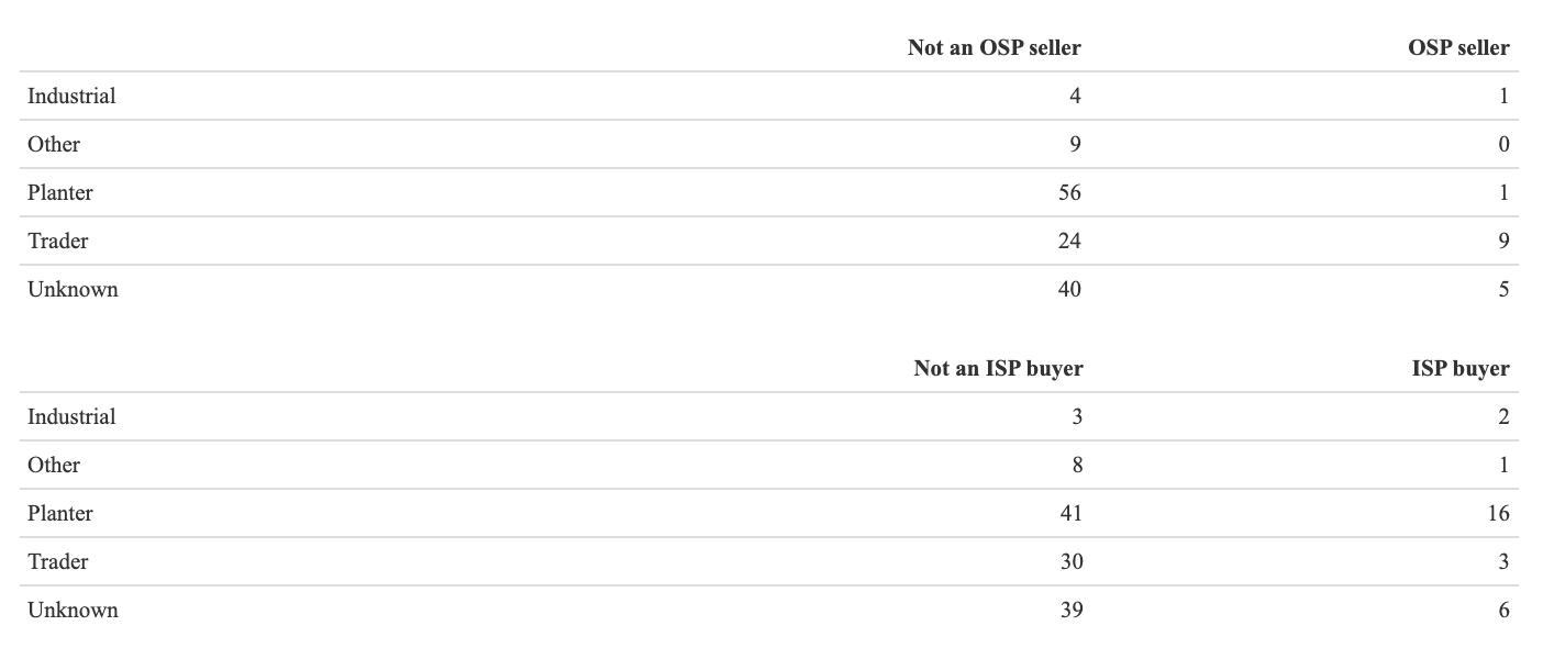
The ISP buyers and OSP sellers are closely linked because they’re trading with each other; if you look again at the shared partners diagram, you’ll see that while the blue nodes have three shared partners, each pair of orange nodes also has two shared partners, in the opposite direction - the blue nodes. This, I think, is historically interesting for two reasons. First, it underscores the point that many actors in the market had clearly-defined roles, which, if not necessarily surprising, at least distinguishes the slave market from more symmetrical networks. But more importantly, it demonstrates the importance of trust. If the most prolific slave traders and plantation owners were closely connected in a network where everyone knew everyone, where prospective customers had information not just about the quality of the slaves they were buying but also about the slave trader that they were buying from, then trust would become profitable; the slave traders had an incentive not to deceive their valuable customers. These relationships could be very strong indeed. On the edge of the network visualisation are two medium-sized blue nodes only connected to each other and nobody else; John L. Manning and William E. Starke. Manning was a plutocratic elder statesman in Southern society; he had been Governor of South Carolina from 1852 to 1854, and according to the 1860 census, he was worth $2,146,000, and owned 670 slaves; he bought 154 of these slaves from Starke on two occasions, May 1859 and April 1860. Starke was primarily a cotton trader, who owned steamships in the Gulf; it seems that he dabbled in human cargo, but perhaps only as a favour to a man from his own social class, for Starke became a brigadier in the Civil War, killed at Antietam while commanding the Stonewall Division. I think that these OSP/ISP structures encode similarly powerful relationships between plantation owners and their trusted merchants.
This bears on one of the great debates in the history of the domestic slave trade: were the slave traders ‘Southern Shylocks’, outcasts from planter society who earned a premium for taking on a job which carried a social stigma; did they, in the famous words of Daniel Hundley, have “a cross-looking phiz, a whiskey-tinctured nose, cold hard-looking eyes, a dirty tobacco-stained mouth, and shabby dress”?24 It’s certainly plausible, as I’ll argue in a later section, that some New Orleans-based speculators cheerfully and regularly engaged in fraud. But interstate traders had regular customers, and couldn’t afford to trick them; the journey, especially overland, from the Old South to New Orleans was so hazardous that only the junior partner in a firm would make the trip, and so the interstate traders needed to be sure that they would have customers waiting for them in New Orleans. For one group of traders, trust was just as valuable an asset as any slave.
Conclusion
The dataset collected by Calomiris and Pritchett collected can’t be used to answer every question about the domestic slave trade; but it can do much more than just index slave prices. In this essay, I’ve tried to do three things: first, I wanted to justify the use of networks in historical analysis; the visualisations and models which I’ve generated demonstrate that this has the potential to be a fruitful approach. Once we think about the New Orleans slave market as a network, it becomes apparent that it has unusual characteristics that distinguish it from the paradigms of network science, and potentially also from slave markets in other times and places. Third, the evidence hints that there may have been several categories of slave traders, who maintained different kinds of business and social relationships with the planter aristocracy. Above all, I’ve tried to approach familiar material with a fresh approach, making the most of modern technology to answer important historical questions.